5  The epidemiological model

The epidemiological model (02_epi_engine.R) is responsible for translating short-term clinical quitting outcomes into long-term, multi-year health outcomes.

Rather than applying static hazard ratios to a fixed patient headcount, the model evaluates the cohort longitudinally. It uses a dynamic Lexis simulation architecture to age patients, apply dynamic risk decay, expand comorbidity profiles, and strictly enforce mortality survival constraints over the defined time horizon.

5.1 The chronological simulation loop

The core of the epidemiological model is its multi-year chronological loop. Rather than calculating a single static cross-section of risk, the model constructs two parallel universes across the time horizon: a Control arm (baseline trajectory) and a Treatment arm (intervention trajectory).

By calculating the precise epidemiological burden in both universes simultaneously, the exact impact of the smoking cessation intervention can be derived from the delta between the two arms.

5.1.1 The dynamic prevalence feedback loop

As the simulation steps forward through time (Year 1, Year 2, Year 3, etc.), it continuously updates the underlying population characteristics. A critical component of this is the dynamic feedback loop governing smoking prevalence.

Before calculating the epidemiological risk for a new year, the model formally transitions successful quitters. It extracts the effective_quits and mathematically shifts this volume of individuals from the current smoker prevalence pool to the former smoker prevalence pool within the Treatment arm. This ensures that the epidemiological benefits compound accurately year-over-year and prevents the double-counting of “at-risk” individuals.

5.1.2 Cohort aging and demographic tracking

As cohorts progress through the Lexis matrix, they naturally age. The simulation accounts for this by recalculating baseline admission rates and background mortality for each advancing year. Consequently, the longitudinal outcomes form a natural curve—the system-wide hospital admissions prevented will ramp up as new treated cohorts enter the simulation, peak, and eventually taper off due to natural aging and background mortality.

5.2 Comorbidity expansion

Patients admitted for a focal condition (e.g., a hip fracture) may carry secondary tobacco-related comorbidities (e.g., COPD or ischaemic heart disease) that also benefit from cessation.

To capture this, the model executes a Cartesian join against a pre-calculated comorbidity_matrix. This expands each unique admission row into a multi-row profile capturing both the focal admission risk and the underlying comorbid event risks.

5.3 Disease mapping and baseline relative risks

To accurately assign epidemiological risk, the model relies on a strict mapping between ICD-10 diagnostic codes, broad disease groups, and published baseline relative risks.

The table below illustrates a subset of the primary conditions modelled, their clinical definitions in Hospital Episode Statistics (HES), and the baseline relative risk (RR) for current smokers (versus never smokers) applied within the engine.

Condition	ICD-10 Lookups	Disease Group (Lag Curve)	Baseline RR (Current Smoker)
Lung Cancer	C33, C34	Cancer	10.92
Larynx Cancer	C32	Cancer	7.01
Chronic Obstructive Pulmonary Disease (COPD)	J40, J41, J42, J43, J44, J47	Respiratory	4.01
Ischaemic Heart Disease	I20, I21, I22, I23, I24, I25	CVD	3.18 (Male 35-64) / 3.93 (Female 35-64)
Ischaemic Stroke	I63, I64, I65, I66, I67	CVD	1.57 (Male) / 1.83 (Female)
Asthma	J45, J46	Respiratory	1.61
Type 2 Diabetes	E11	CVD	1.37

(Note: The full, exhaustive matrix of over 40 conditions is managed dynamically via the disease_mapping_dictionary.csv and input_relative_risks.csv configuration files.)

5.4 Dynamic relative risks and disease-specific decay curves

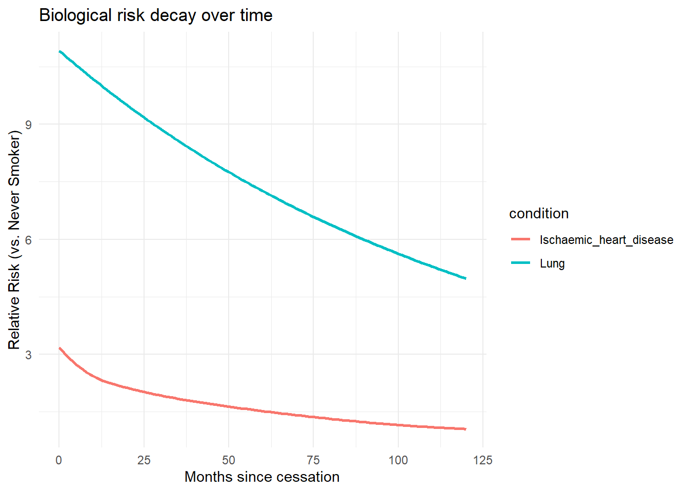
The physiological benefits of smoking cessation do not occur instantaneously. The model incorporates disease-specific risk decay curves to model how relative risk (RR) declines over time following a successful quit attempt.

To translate the discrete follow-up points into a continuous risk trajectory, the data preparation pipeline (00_construct_lags.R) uses a Monotone Hermite spline (monoH.FC). This specific mathematical method is chosen to ensure the risk strictly decreases over time without introducing artificial oscillation.

The model actively audits the alignment of diseases against the input relative risks (input_relative_risks.csv). If an unmapped condition enters the model, a safeguard automatically defaults the relative risk to 1.0 (assuming no cessation benefit) and generates a traceable warning, preventing the simulation from failing silently.

The code allows for the direct visualisation of these input parameters. The following code plots the dynamic relative risks for a 50-64 year old male cohort over a 10-year horizon directly from the model inputs:

Relative risk decay following smoking cessation (Male, 50-64)

5.5 The potential impact fraction (PIF) framework

With the dynamically updated prevalences and the exact time-adjusted relative risks established for the current simulation year, the model uses the potential impact fraction (PIF) (Gunningschepers 1989) to quantify the proportional reduction in disease-specific admissions.

For each demographic stratum and target condition, the model calculates a baseline average relative risk and a new average relative risk (post-intervention). The PIF is calculated as the ratio of the new risk to the baseline risk:

# Extract from 02_epi_engine.R

expanded[, baseline_avg_rr := (prevalence_current * rr_current_agg) +
             (prevalence_former * rr_quitters_agg) + 
             (prevalence_never * rr_never_agg)]

expanded[, new_avg_rr := (new_prev_current * rr_current_agg) +
             (new_prev_former * rr_quitters_agg) + 
             (prevalence_never * rr_never_agg)]

expanded[, pif := fifelse(baseline_avg_rr == 0, 1.0, 
                          new_avg_rr / baseline_avg_rr)]

5.6 Applying mortality survival constraints

Obviously, individuals cannot generate hospital readmissions or incur healthcare costs if they are no longer alive, and so accounting for mortality rates after discharge from hospital is important.

The model merges the cohort with Office for National Statistics (ONS) mortality rates, matched by age, sex, and Index of Multiple Deprivation (IMD) quintile. A survival probability is calculated and applied to the projected admissions:

# Extract from 02_epi_engine.R

expanded[, survival_prob := exp(-mortality_rate * (target_month / 12))]

# Applied dynamically to limit readmissions
temp[, projected_adms := (get(FOCAL_ADMISSIONS) * comorbidity_prob * pif) * survival_prob]

As with the relative risks, an active safeguard checks for missing demographic matches in the mortality tables, defaulting to a zero mortality rate with a warning if unmapped data is detected. By enforcing this mortality constraint, the model mathematically guarantees that admission savings are not falsely claimed for individuals who have died during the follow-up period.